Monte Carlo

1. Introduction

The goal of Monte Carlo method is to calculate the heat transfer between two surfaces. Monte Carlo method uses finite element and probabilist theory.

First, the Monte Carlo method calculates the view factor between two surfaces.

The Monte Carlo method is based on the decomposition of the surfaces (emissive surface \(A_i\) and absorptive surface \(A_j\)) into small finite elements. Here the finite element is triangle.

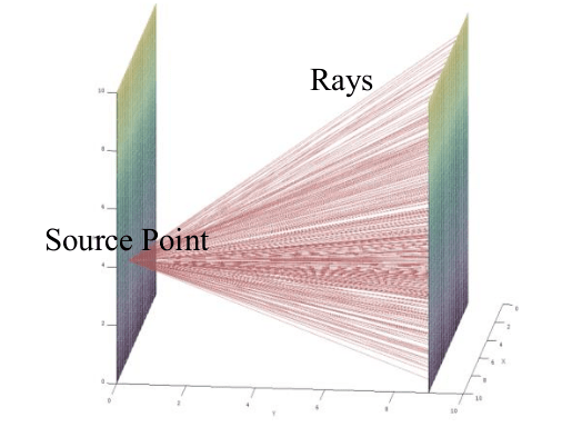
Figure 1. Rays generate by \(A_i\) and intercepted by \(A_j\)

We generate \(N_r\) random rays from \(N_s\) random source points, from emissive element \(e^i_k\). Those rays touch the finite element of absorbent element \(e^j_l\).

The local view factor between element \(e^i_k\) of \(A_i\) and element \(e^j_l\) of \(A_j\) is calculated by subsurface summation :

\[F_{e^i_k \rightarrow e^j_l} = \frac{n}{N} = \frac{n}{N_s N_r}\]

With :

\(N=N_s N_r\) the total number of rays generated by \(A_i\)
\(n\) the number of rays generated by \(A_i\) intercept by \(A_j\)

After the calculation of all local view factors, we can compute the global view factor with equation :

\[F_{A_i \rightarrow A_j} = \frac{1}{A_i} \sum_{k=1}^{K}{ \left( Area(e^i_k) \sum_{l=1}^{L}{F_{e^i_k \rightarrow e^j_l}} \right) }\]

After calculating the view factor, it calculates the heat transfer between surfaces \(A_i\) and \(A_j\), with the formula :

\[q_{A_i \rightarrow A_j} = \sigma F_{A_i \rightarrow A_j} (T_j^4 - T_i^4)\]

With \(T_i\) the absolute temperature of \(A_i\) and \(T_j\) the absolute temperature of \(A_j\).

2. Tools

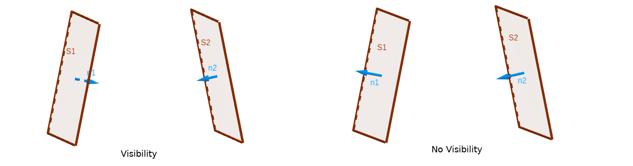
2.1. Visibility of surface

Before calculating the view factor, it is interesting to know if the two surfaces are visible to each other.

For that, we use the oriented normal associated to the elements.

Set oriented surfaces elements \(S_1\) and \(S_2\) (with oriented normal : \(\mathbf{n_1}\) and \(\mathbf{n_2}\)) :

\[S_1 \text{ and } S_2 \text{ are visible } \Longleftrightarrow \mathbf{n_1} \cdot \mathbf{n_2} < 0\]

Figure 2. Visibility between two surface

2.2. Generation of random ray

For the emissive element, we generate some \(N_s\) source point and \(N_r\) ray from one source point.

For that we admit appropriate suppositions on materials :

homogeneous (the emission is the same for any position)
anisotropic (the emission is the same for any direction)

The generation is :

To generate a source point, we randomly choose among the points previously generated in a reference element (for more detail see Choice of Point Source)
Incident angle \(\phi\) of ray follows a uniformly distribution in \([0,2\pi]\)
Azimuthal angle \(\theta\) of ray follows a uniformly distribution in \([0,\pi]\)

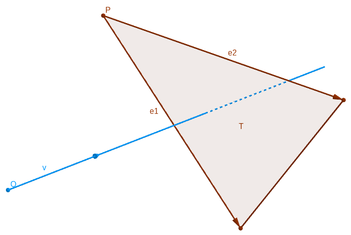
2.3. Interception of ray by triangle

We have the condition for the intersection between a straight line and triangle \(\mathcal{T}\) (of origin point \(P\) and directional vector \(\mathbf{e_1}\) and \(\mathbf{e_2}\)).

Figure 3. Interception of ray by square

\[\text{The ray } \mathcal{C} \text{ is intersept by } \mathcal{T} \Longleftrightarrow \left\{ \begin{eqnarray} \left( \mathbf{v} \wedge \mathbf{e_2} \right) \cdot \mathbf{e_1} \ne 0 \\ 0 \leq \frac{ \vec{OP} \cdot \left( \mathbf{e_2} \wedge \mathbf{v} \right)}{\left( \mathbf{e_2} \wedge \mathbf{v} \right) \cdot \mathbf{e_1} } \leq 1 \\ 0 \leq \frac{ \vec{OP} \cdot \left( \mathbf{e_1} \wedge \mathbf{v} \right)}{\left( \mathbf{e_1} \wedge \mathbf{v} \right) \cdot \mathbf{e_2} } \leq 1 \\ \frac{ \vec{OP} \cdot \left( \mathbf{e_1} \wedge \mathbf{v} \right)}{\left( \mathbf{e_1} \wedge \mathbf{v} \right) \cdot \mathbf{e_2} } + \frac{ \vec{OP} \cdot \left( \mathbf{e_2} \wedge \mathbf{v} \right)}{\left( \mathbf{e_1} \wedge \mathbf{v} \right) \cdot \mathbf{e_2} } \leq 1 \end{eqnarray} \right.\]

3. Algorithm

\begin{algorithm}
    \caption{Calculation of View Factor}
    \begin{algorithmic}
    \FUNCTION{ViewFactor3}{$A_i$, $A_j$, $N_s$, $N_r$}
    \STATE $A_i$ is surface decomposed by $K$ triangles $e^i_k$
    \STATE $A_j$ is surface decomposed by $L$ triangles $e^j_l$
    \STATE $N_s$ number of source point of one element
    \STATE $N_r$ number of ray from one source point

    \STATE $Area_i \leftarrow 0$ : area of surface $A_i$
    \STATE $\Sigma_2 \leftarrow 0$

    \FOR{$e^i_k$ in set of element of surface $A_i$}
        \STATE $\Sigma_1 \leftarrow 0$
        \FOR{$e^j_l$ in set of element of surface $A_j$}
            \IF{\textbf{Visibility}($e^i_k$,$e^j_l$)}
                \STATE $n \leftarrow 0$
                \FOR{$1 \leq i_s \leq N_s$}
                    \STATE $s \leftarrow$ \textbf{SourcePoint}($\mathcal{T}$)
                    \FOR{$1 \leq i_r \leq N_r$}
                        \STATE $r \leftarrow$ \textbf{GenerateRay}($\mathcal{T}$,$s$)
                        \IF{\textbf{Interception}($r$,$e^j_k$)}
                            \STATE $n \leftarrow n + 1$
                        \ENDIF
                    \ENDFOR
                \ENDFOR
                \STATE $F_{e^i_k \rightarrow e^j_l} \leftarrow \frac{n}{N_s N_r}$
            \ENDIF
            \STATE $\Sigma_1 \leftarrow \Sigma_1 + F_{e^i_k \rightarrow e^j_l}$
        \ENDFOR
        \STATE $Area_i \leftarrow Area_i + Area(e^i_k)$
        \STATE $\Sigma_2 \leftarrow \Sigma_2 + Area(e^i_k) \Sigma_1$
    \ENDFOR
    \STATE $F_{global} \leftarrow \frac{1}{Area(A_i)} \Sigma_2$
    \RETURN  $F_{global}$
    \ENDFUNCTION
    \end{algorithmic}
\end{algorithm}

Complexity : \(O\left( K L N_s N_r \right)\), with \(K\) number of elements of \(A_i\), \(L\) number of elements of \(A_j\), \(N_s\) number of source points and \(N_r\) number of rays from one source point.

Complexity more precise :

\[\begin{eqnarray} K \times L \times N_s \times complexity(\mathbf{SourcePoint}) \times N_r \\ \times complexity(\mathbf{Ray}) \times complexity(\mathbf{Interception})] \end{eqnarray}\]

4. Efficiency of method

Discussion of correctness, convergence of the method

References

[Incropera] Fundamentals of Heat and Mass Transfer, Theodore L. Bergman, Adrienne S. Lavine, Frank P. Incropera, David P. DeWitt, Wiley.
[Kumaran1996] Kumaran, M. Kumar, Heat, Air and Moisture Transfer in Insulated Envelope Parts, Final Report, Volume 3.
[Ozturk] Abdurrahman Ozturk, Implementation of View Factor Model and Radiative Heat Transfer Model in MOOSE. University of South Carolina, Download PDF
[Modest] M.F. Modest, Radiative Heat Transfet. Elsevier Science, 2013, ISBN 9780123869906, Chapter 8
[Visionray] Visionaray: A Cross-Platform Ray Tracing Template Library, Zellmann, Stefan and Wickeroth, Daniel and Lang, Ulrich, Proceedings of the 10th Workshop on Software Engineering and Architectures for Realtime Interactive Systems (IEEE SEARIS 2017), 2017
[Visionary::github] Visionaray, Zellman, github.com/szellmann/visionaray