Geometry’s Tools

This page details with the geometry tools needed for the Monte Carlo method.

1. Method of Visionaray

This section describes the geometrical method of Visionary.

1.1. Interception by segment

The question is : When the right $\mathcal{C}$ (of origin $O$ and of direction $\mathbf{v}$) intersects the segment $\mathcal{Q}$ (of vertex $A$ and $B$) ?

Figure 1. Intersection of ray and segment

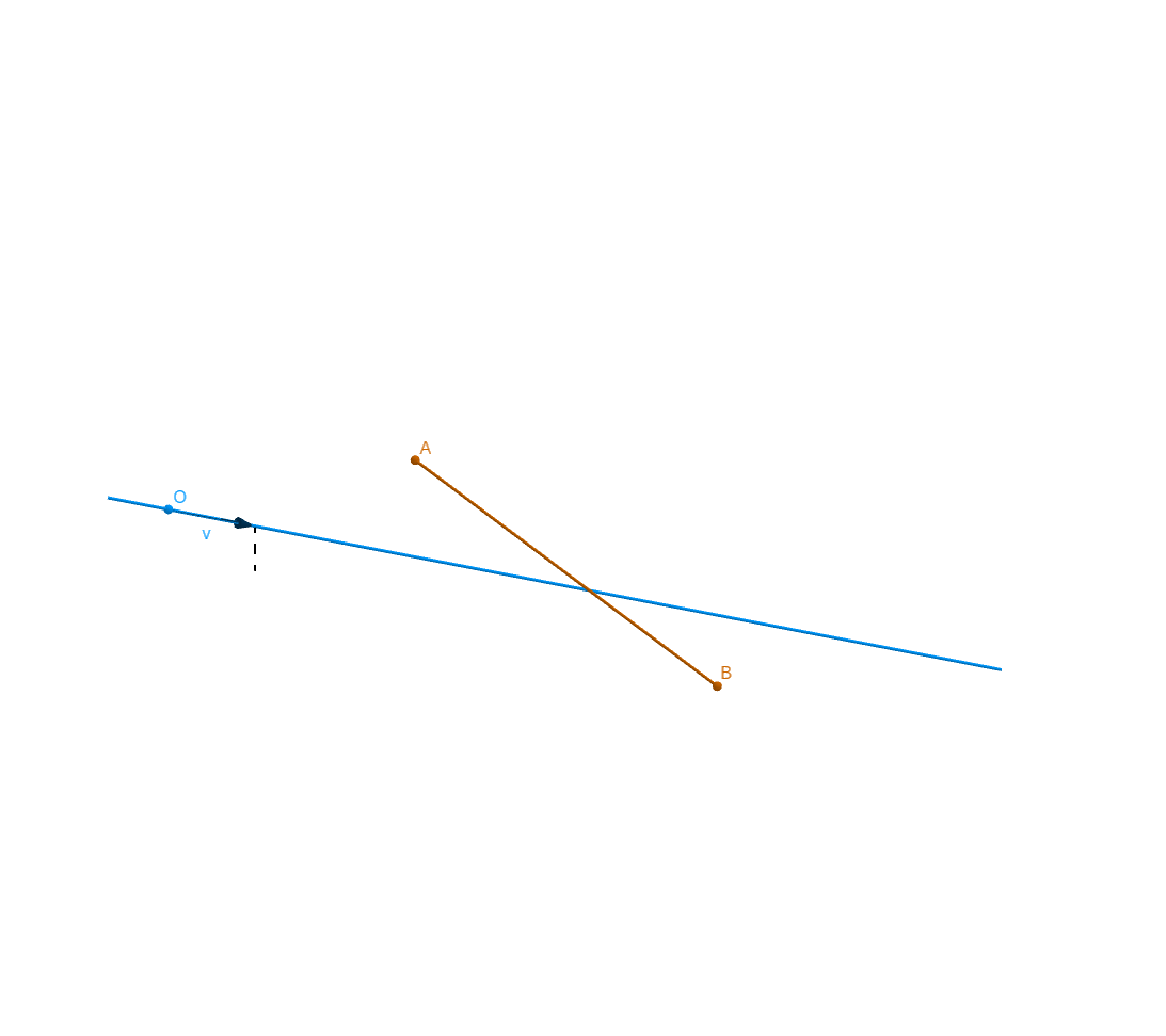
We detail the coordinates :

$A = \begin{pmatrix} x_A \\ y_A \\ z_A \end{pmatrix}$
$B = \begin{pmatrix} x_B \\ y_B \\ z_B \end{pmatrix}$
$\mathbf{v} = \begin{pmatrix} x_v \\ y_v \\ z_v \end{pmatrix}$

We introduce :

$t_1 = \frac{\vec{OA}}{\mathbf{v}}$ (term to term division)
$t_2 = \frac{\vec{OB}}{\mathbf{v}}$

\[\begin{eqnarray} t_{near} &= max \left( min \left( x_{t_1}, x_{t_2} \right), min \left( y_{t_1}, y_{t_2} \right), min \left( z_{t_1}, z_{t_2} \right) \right) \\ t_{far} &= min \left( max \left( x_{t_1}, x_{t_2} \right), max \left( y_{t_1}, y_{t_2} \right), max \left( z_{t_1}, z_{t_2} \right) \right) \end{eqnarray}\]

\[\mathcal{C} \text{ intersect } \mathcal{Q} \Longleftrightarrow t_{near} \leq t_{far}\]

1.2. Interception by triangle

The question is : When the right $\mathcal{C}$ (of origin $O$ and of direction $\mathbf{v}$) intersects the triangle $\mathcal{T}$ (of origin $P$ and of vector $\mathbf{e_1}, \mathbf{e_2}$) ? (we suppose to $O$ not in plan of $\mathcal{T}$)

Figure 2. Intersection of ray and triangle

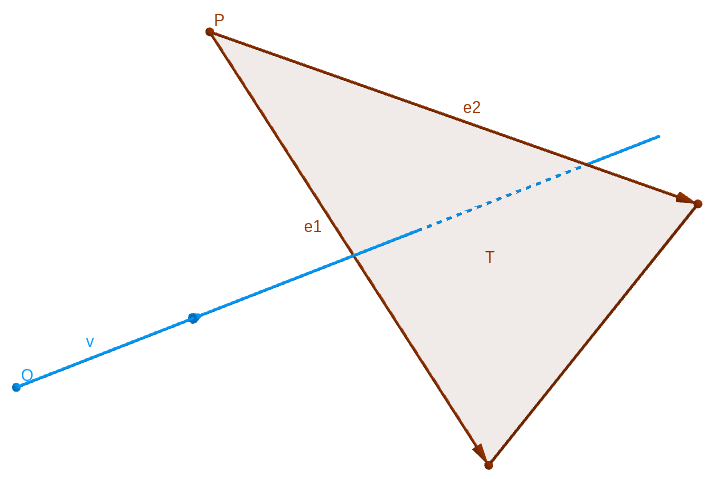
First, we verify if $\mathbf{v}$ is parallel of plan of triangle $\mathcal{T}$ (obviously, if it case, the prolonged right of $\mathcal{C}$ doesn’t intersect $\mathcal{T}$) :

\[\left( \mathbf{v} \wedge \mathbf{e_2} \right) \cdot \mathbf{e_1} = 0 \Leftrightarrow \text{ $\mathbf{v}$ is parallel of plan of triangle $\mathcal{T}$ }\]

Or, the contraposed :

\[\left( \mathbf{v} \wedge \mathbf{e_2} \right) \cdot \mathbf{e_1} \ne 0 \Leftrightarrow \text{ intersection of prolonged right of } \mathcal{C} \text{ and plan of } \mathcal{T} \text{ exists }\]

Remark : $\left( \mathbf{v} \wedge \mathbf{e_2} \right) \cdot \mathbf{e_1} = \left( \mathbf{v} \wedge \mathbf{e_1} \right) \cdot \mathbf{e_2} $

We want $\left( \mathbf{v} \wedge \mathbf{e_2} \right) \cdot \mathbf{e_1} \ne 0$.

Proof : With the rule of calculation of scalar and vectorial produce, we have :

\[\left( \mathbf{v} \wedge \mathbf{e_2} \right) \cdot \mathbf{e_1} = \mathbf{v} \cdot \left( \mathbf{e_2} \wedge \mathbf{e_1} \right)\]

And : $\mathbf{e_2} \wedge \mathbf{e_1}$ is a normal vector of plan of the triangle $\mathcal{T}$.

Thus :

\[\begin{eqnarray} \mathbf{v} \cdot \left( \mathbf{e_2} \wedge \mathbf{e_1} \right) = 0 &\Longleftrightarrow \mathbf{v} \text{ is orthogonal to } \mathbf{e_2} \wedge \mathbf{e_1} \\ &\Longleftrightarrow \mathbf{v} \text{ is parallel to plan of } \mathcal{T} \end{eqnarray}\]

After, we consider to $\mathbf{v} \cdot \left( \mathbf{e_2} \wedge \mathbf{e_1} \right) \ne 0$.

Second, we verify if the intersection is in the triangle $\mathcal{T}$

\[\begin{eqnarray} 0 \leq \frac{\vec{PO} \cdot (\mathbf{v} \wedge \mathbf{e_2})}{ (\mathbf{v} \wedge \mathbf{e_2}) \cdot \mathbf{e_1} } \leq 1 \\ 0 \leq \frac{\vec{PO} \cdot (\mathbf{v} \wedge \mathbf{e_1})}{ (\mathbf{v} \wedge \mathbf{e_1}) \cdot \mathbf{e_2} } \leq 1 \end{eqnarray}\]

Proof : We exprim the space :

\[\begin{eqnarray} &\mathcal{T} = \{ t \mathbf{e_1} + u \mathbf{e_2} + P \in \mathbb{R}^3, 0 \leq t,u \leq 1, u+t \leq 1 \} \\ &\mathcal{C} = \{ O + \lambda \mathbf{v} \in \mathbb{R}^3, \lambda \in \mathbb{R} \} \end{eqnarray}\]

The intersection is :

\[\begin{eqnarray} &Q = \mathcal{T} \cap \mathcal{C} \\ &Q = t \mathbf{e_1} + u \mathbf{e_2} + P = O + \lambda \mathbf{v} \text{ with } 0 \leq t,u \leq 1, u+t \leq 1 \text{ and } \lambda \in \mathbb{R} \end{eqnarray}\]

We want to manipulate the equation :

\[t \mathbf{e_1} + u \mathbf{e_2} + \vec{OP} = \lambda \mathbf{v}\]

\[\begin{eqnarray} \left( t \mathbf{e_1} + u \mathbf{e_2} + \vec{OP} \right) \wedge \mathbf{v} &= \lambda \mathbf{v} \wedge \mathbf{v} = 0 \\ \left( \left( t \mathbf{e_1} + u \mathbf{e_2} + \vec{OP} \right) \wedge \mathbf{v} \right) \cdot \mathbf{e_1} &= 0 \\ \left( t \mathbf{e_1} \wedge \mathbf{v} \right) \cdot \mathbf{e_1} + \left( u \mathbf{e_2} \wedge \mathbf{v} \right) \cdot \mathbf{e_1} + \left( \vec{OP} \wedge \mathbf{v} \right) \cdot \mathbf{e_1} &= 0 \\ t \left( \mathbf{e_1} \wedge \mathbf{e_1} \right) \cdot \mathbf{v} + \left( u \mathbf{e_2} \wedge \mathbf{v} \right) \cdot \mathbf{e_1} + \left( \vec{OP} \wedge \mathbf{v} \right) \cdot \mathbf{e_1} &= 0 \\ 0 + \left( u \mathbf{e_2} \wedge \mathbf{v} \right) \cdot \mathbf{e_1} + \left( \vec{OP} \wedge \mathbf{v} \right) \cdot \mathbf{e_1} &= 0 \\ u = - \frac{\left( \vec{OP} \wedge \mathbf{v} \right) \cdot \mathbf{e_1}}{\left( \mathbf{e_2} \wedge \mathbf{v} \right) \cdot \mathbf{e_1}} \\ u = \frac{ \vec{OP} \cdot \left( \mathbf{e_1} \wedge \mathbf{v} \right)}{\left( \mathbf{e_1} \wedge \mathbf{v} \right) \cdot \mathbf{e_2} } \end{eqnarray}\]

In the same way :

\[t = \frac{ \vec{OP} \cdot \left( \mathbf{e_2} \wedge \mathbf{v} \right)}{\left( \mathbf{e_2} \wedge \mathbf{v} \right) \cdot \mathbf{e_1} }\]

Thus, we have the condition :

\[\left\{ \begin{eqnarray} 0 \leq t &= \frac{ \vec{OP} \cdot \left( \mathbf{e_2} \wedge \mathbf{v} \right)}{\left( \mathbf{e_2} \wedge \mathbf{v} \right) \cdot \mathbf{e_1} } \leq 1 \\ 0 \leq u &= \frac{ \vec{OP} \cdot \left( \mathbf{e_1} \wedge \mathbf{v} \right)}{\left( \mathbf{e_1} \wedge \mathbf{v} \right) \cdot \mathbf{e_2} } \leq 1 \\ t+u &= \frac{ \vec{OP} \cdot \left( \mathbf{e_1} \wedge \mathbf{v} \right)}{\left( \mathbf{e_1} \wedge \mathbf{v} \right) \cdot \mathbf{e_2} } + \frac{ \vec{OP} \cdot \left( \mathbf{e_2} \wedge \mathbf{v} \right)}{\left( \mathbf{e_1} \wedge \mathbf{v} \right) \cdot \mathbf{e_2} } \leq 1 \end{eqnarray} \right.\]

Recapitulation :

\[\text{The ray } \mathcal{C} \text{ is intersept by } \mathcal{T} \Longleftrightarrow \left\{ \begin{eqnarray} \left( \mathbf{v} \wedge \mathbf{e_2} \right) \cdot \mathbf{e_1} \ne 0 \\ 0 \leq \frac{ \vec{OP} \cdot \left( \mathbf{e_2} \wedge \mathbf{v} \right)}{\left( \mathbf{e_2} \wedge \mathbf{v} \right) \cdot \mathbf{e_1} } \leq 1 \\ 0 \leq \frac{ \vec{OP} \cdot \left( \mathbf{e_1} \wedge \mathbf{v} \right)}{\left( \mathbf{e_1} \wedge \mathbf{v} \right) \cdot \mathbf{e_2} } \leq 1 \\ \frac{ \vec{OP} \cdot \left( \mathbf{e_1} \wedge \mathbf{v} \right)}{\left( \mathbf{e_1} \wedge \mathbf{v} \right) \cdot \mathbf{e_2} } + \frac{ \vec{OP} \cdot \left( \mathbf{e_2} \wedge \mathbf{v} \right)}{\left( \mathbf{e_1} \wedge \mathbf{v} \right) \cdot \mathbf{e_2} } \leq 1 \end{eqnarray} \right.\]

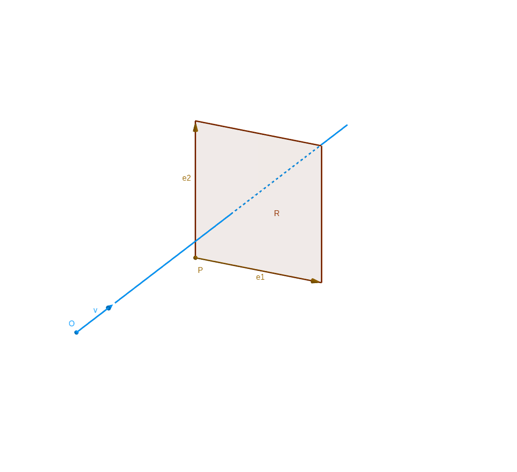
1.3. Interception by parallelogram

We can adapt the recapitulation to have the intersction between right and parallelogram $\mathcal{R}$ (of origin point $P$ and directional vector $\mathbf{e_1}$ and $\mathbf{e_2}$)

Figure 3. Intersection of ray and square

\[\text{The ray } \mathcal{C} \text{ is intersept by } \mathcal{R} \Longleftrightarrow \left\{ \begin{eqnarray} \left( \mathbf{v} \wedge \mathbf{e_2} \right) \cdot \mathbf{e_1} \ne 0 \\ 0 \leq \frac{ \vec{OP} \cdot \left( \mathbf{e_2} \wedge \mathbf{v} \right)}{\left( \mathbf{e_2} \wedge \mathbf{v} \right) \cdot \mathbf{e_1} } \leq 1 \\ 0 \leq \frac{ \vec{OP} \cdot \left( \mathbf{e_1} \wedge \mathbf{v} \right)}{\left( \mathbf{e_1} \wedge \mathbf{v} \right) \cdot \mathbf{e_2} } \leq 1 \end{eqnarray} \right.\]

1.4. Interception by plan

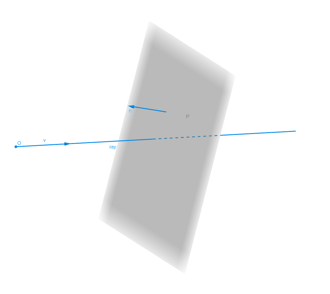
\[\text{ the semi-right $\mathcal{C}$ (of origin $O$ and direction $\mathbf{v}$) intersect the plan $\mathcal{P}$ (of normal $\mathbf{n}$) } \Longleftrightarrow \mathbf{v} \wedge \mathbf{n} \ne 0\]

Figure 4. Intersection of ray and plan

Proof : We have

\[\begin{eqnarray} \mathcal{C} \text{ intersect } \mathcal{P} &\Longleftrightarrow& \mathbf{v} \text{ not parallel to } \mathbf{n} \\ &\Longleftrightarrow& \mathbf{v} \wedge \mathbf{n} \ne 0 \end{eqnarray}\]

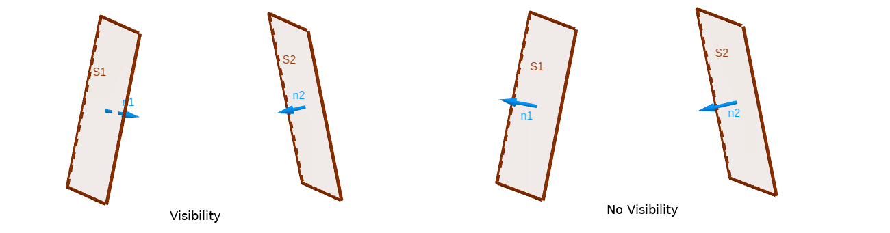
2. Visibility between two plan

Before to calculate the view factor between two surfaces, we must know if they are visible from each other.

We must define an oriented surface, which side of the surface emits and which one absorbs.

Example 1. Definition of oriented surface

An oriented surface is a surface (suppose contain in plan), is a surface with an oriented normal.

Set oriented surfaces $S_1$ and $S_2$ (with oriented normal : $\mathbf{n_1}$ and $\mathbf{n_2}$) :

\[S_1 \text{ and } S_2 \text{ are visible } \Longleftrightarrow \mathbf{n_1} \cdot \mathbf{n_2} < 0\]

Figure 5. Visibility between two surface

3. Convertion cartesian/polar

References

[Incropera] Fundamentals of Heat and Mass Transfer, Theodore L. Bergman, Adrienne S. Lavine, Frank P. Incropera, David P. DeWitt, Wiley.
[Kumaran1996] Kumaran, M. Kumar, Heat, Air and Moisture Transfer in Insulated Envelope Parts, Final Report, Volume 3.
[Ozturk] Abdurrahman Ozturk, Implementation of View Factor Model and Radiative Heat Transfer Model in MOOSE. University of South Carolina, Download PDF
[Modest] M.F. Modest, Radiative Heat Transfet. Elsevier Science, 2013, ISBN 9780123869906, Chapter 8
[Visionray] Visionaray: A Cross-Platform Ray Tracing Template Library, Zellmann, Stefan and Wickeroth, Daniel and Lang, Ulrich, Proceedings of the 10th Workshop on Software Engineering and Architectures for Realtime Interactive Systems (IEEE SEARIS 2017), 2017
[Visionary::github] Visionaray, Zellman, github.com/szellmann/visionaray
Méthode Numérique pour le EDP, Christophe Prudhomme, feelpp.github.io/csmi-edp/#/, Programmation de le méthode élément fini, Formule de quadrature
CEMOSIS, CEMOSIS, www.cemosis.fr/
L’Accord de Paris, unfccc.int/fr/process-and-meetings/the-paris-agreement/l-accord-de-paris, UNFCC Sites and platforms
[Infographie] Énergie : quel secteur d’activité consomme le plus ?, www.gazprom-energy.fr/gazmagazine/2017/09/consommation-energetique-secteur-activite/, Gazprom Energy
L’électricité dans le secteur résidentiel, www.edf.fr/groupe-edf/espaces-dedies/l-energie-de-a-a-z/tout-sur-l-energie/le-developpement-durable/l-electricite-dans-le-secteur-residentiel, EDF
Synapse Concept, www.synapse-concept.com/
4fastsim-ibat, www.cemosis.fr/projects/4fastsim-ibat/
Feel++ Docs, docs.feelpp.org/feelpp/index.html